Boiling

Rohsenow Boiling

The empirical standard pool boiling correlation [632] is used to model liquid film boiling at a hot wall. The film starts to boil when the wall temperature exceeds the boiling temperature of the liquid. The heat flux passing from the wall to the film increases in proportion to the cubic power of $\Delta T_W=T_W-T_{\mathrm{sat}}$ as:

where:

• the viscosity ${\mu }_f$ , the Prandtl number ${{\text{Pr}}_f}^n$ , and the specific heat $C_{p,f}$ are evaluated for the liquid phase.
• ${\rho }_f$ and $\rho$ denote the densities of the liquid and gas phases.
• $g$ and $\sigma$ denote the gravity acceleration and surface tension coefficient respectively.
• $c_{sf}$ and $n$ characterize the fluid wall interface.

  For example, for water-brass contact, the values are $c_{sf}=0.006$ and $n=3$ .

• $T_{\mathrm{sat}}$ represents the saturation temperature of the mixture and is computed from the temperature-dependent saturation pressure of its components by applying Dalton’s law.

The heat flux increases as $T_W$ increases but does not exceed a critical heat flux that is:

where $c_{\max }=0.15$ . After $q_{\max }$ has been attained, the heat flux decreases to its minimum at the Leidenfrost temperature $T_L$ :

where $c_{\min }=0.09$ .

The wall temperature of maximal heat flux $T_S=T_{\mathrm{sat}}+{\mathrm{\Delta T}}_S$ can be obtained from equations Eqn. (2802) and Eqn. (2803), resulting in:

Based on this correlation, the heat flux from the wall is computed as follows:

$\Delta T_L=T_L-T_{\mathrm{sat}}$ and $c_s$ is assumed to be 1.2.

The component mass rates of vaporization are then computed as

where $c_e$ is the wall boiling evaporation factor that determines how much of the boiling heat flux generates vapor. A value smaller than one means that a portion of the boiling heat flux does not generate vapor but heats up the film, for example:

• when heat is supplied near the wall to bubbles which then move away into the liquid film and condense into the film
• when evaporation takes place at the base of a bubble and condenses at its tip.

Bulk Boiling

The heat transfer to the interface between the phases is used to compute the rate of evaporation.

For the Rohsenow boiling model, Simcenter STAR-CCM+ calculates the mass rate of evaporation from:

$${\dot{m}}_v=\frac{\text{HTCxArea}\left(T-T_{\mathrm{sat}}\right)}{\Delta H^{\mathrm{vap}}}$$

(2808)

assuming that:

• The vapor bubbles are at the saturation temperature.
• The temperature of the liquid is approximately the temperature of the mixture.
• All the heat flux from the liquid to the interface is used in mass transfer due to evaporation.

$\text{HTCxArea}$ is the product of the heat transfer coefficient between the vapor bubbles and the surrounding liquid, and the specific contact area (contact area per unit volume) between the two. $\mathrm{\Delta }{H}^{\mathrm{vap}}$ is the latent heat of vaporization of the mixture:

$$\mathrm{\Delta }{H}^{\mathrm{vap}}={\sum }_i^{}{Y}_i{{\mathrm{\Delta H}}_i}^{\mathrm{vap}}$$

(2809)

where $Y_i$ is the mass fraction and ${{\mathrm{\Delta H}}_i}^{\mathrm{vap}}$ is the latent heat of pure component $i$ . This latent heat is the difference between the enthalpy of its liquid phase $H_{i,f}$ and its gas phase $H_i$ .

$${{\mathrm{\Delta H}}_i}^{\mathrm{vap}}=H_i-H_{i,f}$$

(2810)

Habchi Boiling

The Habchi boiling model calculates the vaporization of liquid films across both nucleate and transition boiling regimes. Additionally, the Habchi boiling model considers the effects of ambient gas pressure and wall roughness when calculating the liquid evaporation rate.

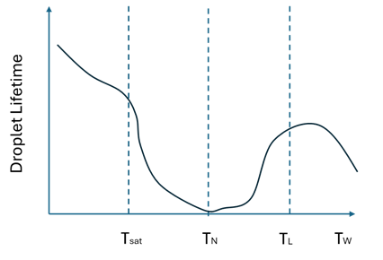
The Habchi boiling approach uses the saturation, Nukiyama, and Leidenfrost temperatures to differentiate between the fluid film boiling regimes.

• Below the saturation (boiling) temperature, when ${𝑇}_{𝑤}<{𝑇}_{𝑠𝑎𝑡}$ , the heat flux is low, and evaporation occurs to some extent.
• When ${𝑇}_{𝑠𝑎𝑡}<{𝑇}_{𝑤}<{𝑇}_{𝑁}$ ​, vapor cavities form around nucleation sites on the wall. The maximum heat flux is reached at the Nukiyama temperature ${𝑇}_{𝑁}$ .
• For ${𝑇}_{𝑁}<{𝑇}_{𝑤}<{𝑇}_{𝐿}$ ​, above the Nukiyama temperature, vapor pockets coalesce to form a cushion, which reduces the contact of the liquid with the wall, thus slowing conduction.
• When ${𝑇}_{𝑤}>{𝑇}_{𝐿}$ ​, in the Leidenfrost regime, the presence of the vapor cushion further slows conduction.

At high wall temperatures, the film rapidly heats up and boils away. As a result, when the film thickness approaches zero, Simcenter STAR-CCM+ limits the maximum film temperature to the wall temperature to ensure that a defined zero thickness film behaves as if there was no film. If any film remains and boiling occurs, the film temperature remains below ${𝑇}_{𝑠𝑎𝑡}$ .

The thermal boundary height can be calculated by using the maximum evaporation rate $\stackrel{\mathrm{.}}{m_{CHF}}$ (at critical heat flux or Nukiyama temperature) and the latent heat at saturation temperature $L_{sat}$ , obtained as:

where:

and:

• $h_f$ is the film thickness.
• $\theta$ is the contact angle.
• $c_{lld}^{\max }$ is the maximum length of the contact lines of the liquid film.
• $k_{clld}$ is a dimensionless length density of contact lines, defined as:

  $$k_{clld}\left(T_W\right)=(1-k_{clld}^{\min }{T}_{**}+k_{clld}^{\min })$$

  (2822)
  and $T_{**}=\frac{{T_L-T}_W}{\Delta T_L}$ .
• $k_{clld}^{\min }$ is the minimum dimensionless length density of contact lines.

Nukiyama and Leidenfrost Temperature

where:

• $T_c$ is the critical temperature. For multi-component liquid this is the highest of the critical temperatures of the liquid components.
• $P$ is pressure.
• $A$ is $A=\max (1,T_{cr|1bar}-T_c)$ .
• $T_b$ is the normal boiling temperature at 1 atm. For a multi-component liquid, choose $T_b$ as a function of composition.

If there are no experimental data available, the Nukiyama temperature is estimated it to be halfway between the film saturation temperature and the Leidenfrost temperature: