Electrochemical Surface Reactions (Heterogeneous)

A general form of electrochemical surface reactions is represented as:

where $\eta$ is the surface overpotential.

where ${\nu }_i$ is the stoichiometric coefficient of the reaction component, ${\nu }_e$ is the stoichiometric coefficient of the electron, and $F$ is Faraday's constant.

where $PIAD$ is the phase interaction area density in dimension 1/Length.

where ${\varphi }_s$ represents the potential of the conductor, ${\varphi }_l$ represents the potential of the electrolyte relative to a reference electrode, $U_{eq}$ is the equilibrium potential, $j_{n,s}$ is the boundary-specific electric current, and $R$ is the resistance that is specified at the boundary or interface.

${\varphi }_l$ is generally obtained from the Electrodynamic Potential model. For electrochemically reacting boundaries, ${\varphi }_s$ is specified in the physics values at each boundary, whereas it is also determined from the Electrodynamic Potential model in the case of an interface or a region when the porous media model is used.

where $\varphi$ is the electric potential.

The driving force behind these reactions is the difference in Gibbs free energy $\Delta G°$ between the reactants and the products—which equates to the equilibrium potential $U_{eq}$ . For the electrochemical reaction:

The potential difference $U$ at the interface is due to the difference in potential of the metal and the electrolyte.

In Simcenter STAR-CCM+, the potential difference is defined as:

where ${\varphi }_s$ is the potential of the conductor and ${\varphi }_l$ is the potential of the electrolyte.

The overpotential definition is equivalent to that of the overpotential which is defined for the electrodynamic potential model in Eqn. (4295) where:

• ${\varphi }_s$ is equivalent to ${\varphi }_1$

  This value represents the potential of the boundary on the conductor region side of the interface which corresponds to the second boundary that you select when defining an interface.

• ${\varphi }_l$ is equivalent to ${\varphi }_0$

  This value represents the potential of the boundary on the electrolyte region side of the interface which corresponds to the first boundary that you select when defining an interface.

• ${\varphi }_E$ represents the equilibrium potential $U_{eq}$ .

If the potential difference at the interface is larger than the equilibrium potential, $U>U_{eq}$ , the reaction is anodic. If the potential difference is less than the equilibrium potential, $U<U_{eq}$ , the reaction is cathodic. When the equilibrium potential is zero, the anodic and cathodic reactions balance, and the net flux is zero.

Anodic reactions (that produce electrons) are related to positive overpotential. Cathodic reactions (that consume electrons) are related to negative overpotential. In these reactions, the current density $i$ is positive for anodic reactions and negative for cathodic reactions.

The flow of charged particles determines the current (electrons in the metal and ions in the electrolyte).

In each of these reaction formulation property methods, temperature $T$ is essential to parameterize the rates of electrochemical reactions. In particular, temperature influences the equilibrium potential $U_{eq}$ when it is specified using the Nernst Equilibrium Potential method. When either the gas, liquid, multicomponent gas, or multicomponent liquid model is selected, the temperature is determined by the energy models that are selected. If no energy model is selected, Simcenter STAR-CCM+ uses a constant temperature of 293.15K. However, when one of the Multiphase models is selected, the temperature is calculated as follows:

Butler-Volmer

When a reaction is reversible, both anodic and cathodic Tafel equations are combined to form the Butler-Volmer equation:

$$j=j_o\left\{\text{exp }\left({\alpha }_a\frac{F}{R_{u}T}\eta \right)-\text{exp}\left(-{\alpha }_c\frac{F}{R_{u}T}\eta \right)\right\}$$

(4128)

where ${\alpha }_a$ and ${\alpha }_c$ are the anodic and cathodic charge transfer coefficients respectively.

${\alpha }_a$ and ${\alpha }_c$ consider the apparent charge transfer coefficient—they are the intrinsic transfer coefficients that are multiplied by the number of electrons ${\nu }_e$ that are involved in the reaction.

The exchange current density and the equilibrium potential often depend on other variables such as concentrations of reactants and products, temperature, and surface contaminants. Using Butler-Volmer kinetics, the specific reaction current is expressed as:

$$j_{n,s}=j_0\cdot \underset{i}{\mathrm{\Pi }}{\left(\frac{c_i}{c_{i,ref}}\right)}^{{\gamma }_i}(e^{\frac{{\alpha }_{a}F\eta }{R_{u}T}}-e^{\frac{-{\alpha }_{c}F\eta }{R_{u}T}})$$

(4129)

where:

$$e^{\frac{{\alpha }_{a}F\eta }{R_{u}T}}$$

(4130)

accounts for anodic currents that are directed from the solid towards the liquid and:

$$e^{\frac{-{\alpha }_{c}F\eta }{R_{u}T}}$$

(4131)

accounts for cathodic currents that are directed from the liquid towards the solid. The product term $\underset{i}{\mathrm{\Pi }}{\left(\frac{c_i}{c_{i,ref}}\right)}^{{\gamma }_i}$ multiplies the molar concentrations of reactants or products that are taking part in the reaction to the power of the rate exponent ${\gamma }_i$ . You can specify ${\gamma }_i$ for each reactant and product in the reaction. $c_{i,ref}$ represents a reference concentration for species $i$ , $c_{i,ref}$ is 1 kmol/m³. The following diagram shows the dependence of the specific reaction current $j_{n,s}$ on the surface overpotential $\eta$ for the Butler-Volmer method. Splitting the specific reaction current into anodic and cathodic contributions illustrates the nature of Tafel reactions.

Tabular

The Tabular Polarization Curve method allows you to simulate electrochemical reactions using tabular data that defines the current and electrochemical potential at the interface between the metal and the electrolyte. The Tabular method lets you import polarization curves when modeling species that do not follow the same pattern as generalized by the Butler-Volmer equation.

When modeling corrosion, Simcenter STAR-CCM+ uses the polarization curves to calculate the corrosion potential for each metal when the current is zero.

When this method is selected, you set the boundary conditions at the interface between the metal and the electrolyte manually. See Tabular Polarization Curve Properties.

Tafel

Butler-Volmer kinetics accounts for both anodic reactions in which free electrons are produced in the solid phase, and cathodic reactions in which free electrons are consumed. In some scenarios, if one of the apparent transfer coefficients is small or operates solely in either positive or negative surface overpotential conditions, reactions can exhibit currents in only anodic or cathodic directions. In such cases, either $j_a$ or $j_c$ is neglected and the negligible reaction term is disregarded. The specific reaction current $j_{n,s}$ then reads:

$$j_{n,s}=\pm j_0\cdot \underset{i}{\mathrm{\Pi }}{\left(\frac{c_i}{c_{i,ref}}\right)}^{{\gamma }_i}\cdot e^{\left(\frac{\pm \alpha \cdot F_{\eta }}{R_{u}T}\right)}$$

(4132)

Since the apparent transfer coefficient $\alpha$ is no longer specified as anodic or cathodic, when using the Electrochemical Species model, the reaction setup determines the direction of the current ( $\pm$ ).

• When electrons are specified as reactants, the current is cathodic ( $-\alpha$ )
• When electrons are specified as products, the current is anodic ( $+\alpha$ )

In the absence of the Electrochemical Species model, the direction of the current is specified in the Properties of the Reaction Formulation > Tafel node, see Reaction Formulation.

Tafel Slope (log 10)

The Tafel equation is often laid out and parameterized as it is in the Butler-Volmer section, with both exponent variables independent of electric potential. In practice, often these exponent variables are measured as one combined quantity, $\beta$ , and called the Tafel Slope:

$$\beta =\ln \left(10\right)\frac{R_{u}T}{\alpha F}=\pm 2.303\frac{R_{u}T}{\alpha F}$$

(4133)

so the specific reaction current is expressed as:

$$j_{n,s}=\pm j_0\cdot \underset{i}{\mathrm{\Pi }}{\left(\frac{c_i}{c_{i,ref}}\right)}^{{\gamma }_i}\cdot {10}^{\left(\frac{\eta }{\beta }\right)}$$

(4134)

When specifying the y-intercept value for the specific exchange current density, ${\log }_{10}\left(j_0\right)$ , the specific reaction current is expressed as:

$${\log }_{10}\left(\left|j_{n,s}\right|\right)={\log }_{10}\left(j_0\right)+{\log }_{10}(\underset{i}{\mathrm{\Pi }}{\left(\frac{c_i}{c_{i,ref}}\right)}^{{\gamma }_i})+\frac{\eta }{\beta }$$

(4135)

You can specify the combined term $\beta$ as a scalar profile.

Since $\beta$ is not specified as anodic or cathodic, the Electrochemical Species model determines the direction of the current ( $\pm$ ). In the absence of the Electrochemical Species model, the direction of the current ( $\pm$ ) is set in the Properties of the Reaction Formulation > Tafel Slope (log 10) node, see Reaction Formulation.

Transport Limited Tafel Slope (log 10)

The Transport Limited Tafel Slope method approximates effects that are not initially accounted for in the simulation setup. When a positive limiting current $j_{\lim }$ is specified, the specific reaction current that is provided by the Tafel method (Eqn. (4132)) is limited:

$$j_{n,s}=\frac{1}{\frac{1}{j_{\lim }}+\frac{1}{j_{tafel}}}$$

(4136)

This method of modeling is empirical and is not based on first principles.

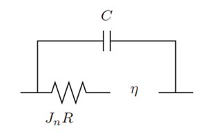
Double Layer Capacitance

The reaction formulation methods calculate the faradaic electric current density that result from electrochemical reactions. As a consequence of ion and electron attraction or repulsion, electric charges accumulate on the reaction site between the electrode and electrolyte, causing transient (non faradaic) capacitive electric currents. The impact of this phenomenon is modeled with a double layer capacitor that is connected in parallel to the main electrochemical reaction site. In transient mode, this configuration creates an additional double layer capacitance electric current density over the electrochemical reaction site.

Nernst Equilibrium Potential

When the equilibrium potential $U_{eq}$ is specified using the Nernst Equilibrium Potential method, $U_{eq}$ is computed as:

$E^0$ is the Nernst Standard Potential at the reference molar concentration of unity.

Nernst Equilibrium Potential from Thermodynamic Data

When the equilibrium potential $U_{eq}$ is specified using the Nernst Equilibrium Potential from Thermodynamic Data method, $U_{eq}$ is computed as:

in which $T$ is temperature, ${\nu }_e$ is the stoichiometric coefficient of electrons, and ${\nu }_i$ is the stoichiometric coefficient of reactant species $i$ . ${\nu }_i$ and ${\nu }_e$ is positive for species/electrons that are reactants, and negative for species/electrons that are products. $side$ has a value of 1, except at interfaces when ionic species reside on the solid side of the interface, then $side$ has a value of -1.

Electrochemical Reaction Heating

The Electrochemical Reaction Heating model accounts for heat contributions which are due to reversible and irreversible electrochemical processes (for heat contributions due to sorption, see Eqn. (4174)). This feature is important for applications such as electroplating or solid oxide fuel cells which create high electrochemical currents.

where, for the Butler-Volmer method, the irreversible heat contribution is always positive:

$j_{n,s,i}$ represents the boundary specific electric current density on the solid for species $i$ , ${\eta }_i$ is the surface overpotential for species $i$ , and $j_{n,s,i}T\frac{d{U}_{eq}}{dT}$ represents the reversible heat contribution.

For Eulerian multiphase, the specific electrochemical reaction heat surface source term contributions ${\dot{q}}_A$ from each phase is expressed as:

where $\alpha$ is the volume fraction of phase $i$ for each side of the interface/boundary, and $j_{n,s}$ is the specific reaction current that is provided by the Butler-Volmer method, Eqn. (4129).