Setting Photon Monte Carlo Solver Parameters

Given the statistical nature of the solver, accuracy increases with the number of photon bundles used in the simulation. For this reason, you increase the average number of rays (photon bundles) traced from each patch.

To set the parameters:

Select the Solvers > Photon Monte Carlo > Ray Tracing Parameters node and set Rays Per Patch to 25.

The SPMC model allows for aggregating the statistics over iterations via the use of a statistical sampling factor. This ensures that you do not have to use a large number of rays in the SPMC computations, and the statistics for the radiative quantities of interest can be aggregated over several iterations. At a value of 1, the aggregated solution is set to the latest SPMC ray tracing solution. For a value of 0.5, the aggregated solution is updated by taking half of the latest solution and half of the previous aggregated solution. A value of 0 means that the aggregated solution stays unchanged.

You are advised to use a high sampling factor at the start of the simulation, since that leads to a fast feedback of radiative solutions into the energy equation and, consequently, a fast evolution of the temperature field.

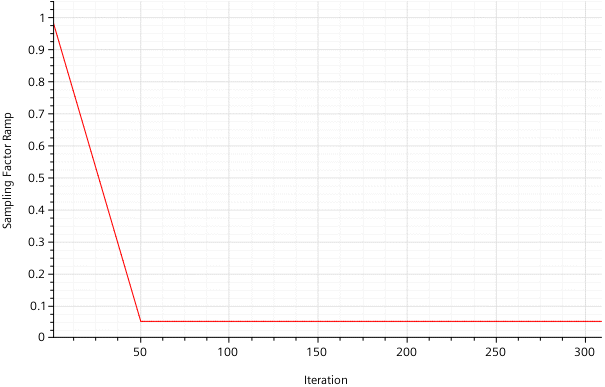
For this tutorial, you set up a linear ramp that starts with a sampling factor of 1.0, reduces to a value of 0.05 during the first 50 iterations, and then remains constant until the simulation completes:

Set up the ramp:
1. Expand the Reports node and create a new New > User > Expression report.
2. Rename the Expression 1 report to Sampling Factor Ramp.
3. Select the Sampling Factor Ramp node and set Definition as follows:
  ${Iteration}<${Sampling Factor Ramp Duration} ? ${Initial Sampling Factor} - (${Initial Sampling Factor}-${Final Sampling Factor})/${Sampling Factor Ramp Duration}*${Iteration}: ${Final Sampling Factor}
  
  See Appendix: Parameters.
4. Select the Solvers > Photon Monte Carlo > Statistical Sampling Factor node and set Sampling Factor to ${Sampling Factor Ramp}.
To visualize the sampling factor ramp during the run, you monitor the created report and add it to the pre-defined temperature plot:
1. Right-click the Reports > Sampling Factor Ramp node and select Create Monitor from Report.
2. Right-click the Plots > Min/Max Temperature Plot > Data Series node and select Add Data.
3. In the Add Data Providers to Plot dialog, select Sampling Factor Ramp Monitor and click OK.
4. Select the Data Series > Sampling Factor Ramp Monitor node and set Y-Axis to Right Axis.

By default, the SPMC calculations are invoked at every iteration. However, the temperature field often undergos small changes from iteration to iteration. To reduce computational cost for this tutorial, you perform the SPMC computations only every fifth iteration:

Select the Solvers > Photon Monte Carlo > Update Frequency > Steady node and set Iteration Update Frequency to 5.
Save the simulation .