Setting Up Anisotropic Linear Forcing
Setting up the Anisotropic Linear Forcing method for a scale-resolving simulation requires a preliminary RANS simulation. You transfer the Reynolds-averaged velocity and turbulence variables to your scale-resolving simulation and apply the values inside a specific forcing volume. When you run the scale-resolving simulation, the ALF method forces the mean properties of the scale-resolving simulation in the forcing volume towards the Reynolds-averaged values.
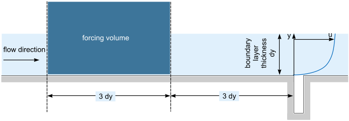
Example: To model the boundary layer flow over a cavity, you place the forcing volume about three local boundary layer thicknesses upstream of the cavity and size the forcing volume about three local boundary layer thicknesses long.

- Perform a preliminary RANS simulation—either on the same simulation domain as the scale-resolving simulation or on a subset of the simulation domain that corresponds to the forcing volume. The RANS simulation provides you with the velocity and turbulence fluctuations towards which you want to force the mean properties of your scale-resolving simulation.
-
Extract and export the velocity components (Velocity.i,
Velocity.j,
Velocity.k) and one of the following combinations of field functions to a
Table (x,y,z):
- Turbulent Kinetic Energy and Turbulent Dissipation Rate
- Reynolds Stresses and Turbulent Dissipation Rate
- Turbulent Kinetic Energy and a user field function that defines the turbulent length scale of the used RANS model (see Turbulent Time, Length, and Velocity Scales)
- Reynolds Stresses and a user field function that defines
For certain RANS models, these field functions are not available by default. You must turn on temporary storage for the corresponding turbulence solver to access these field functions. See Turning on Temporary Storage. - Set up your scale-resolving simulation and add the Anisotropic Linear Forcing model to the physics continuum. See Anisotropic Linear Forcing Model Reference.
- Import the table that you exported in Step 2 in your scale-resolving simulation. See Reading a Table Data File.
-
For the region where you want to apply the forcing, set
to one of the following:
- K + Length Scale
- K + Epsilon
- Reynolds Stress + Length Scale
- Reynolds Stress + Epsilon
You choose the option according to your exported RANS data. For example, for Turbulent Kinetic Energy and Turbulent Dissipation Rate, you choose K + Epsilon. -
Depending on the selected option, set the corresponding
to the imported table values.
For example, for K + Epsilon, you set the following values:
- ALF Velocity
- ALF Turbulent Kinetic Energy
- ALF Dissipation Rate
-
Select the
ALF Blending Function node and set the properties depending on the extent of your ALF volume:
Extent of ALF Volume Steps Whole region Set ALF Blending Function to a constant value of 1. Portion of the region - Create a user field function that is equal to 1 in the ALF volume and 0 elsewhere.
Example: ($$Position[0]<=1)?1:0 assigns all cells with the centroid x component smaller than 1 to the forcing volume.
- Set ALF Blending Function to the created user field function.
- Create a user field function that is equal to 1 in the ALF volume and 0 elsewhere.
-
Create a volume integral report and set the following properties:
Property Setting Field Function ALF Momentum Source Term Parts Set the region where you apply the forcing. See Reporting Results.
- Create a monitor and plot from the created report. See Monitoring the Solution and Plotting Results.
- Run the simulation.
-
In the physics continuum, select the
Anisotropic Linear Forcing node and adjust the number of iterations as follows:
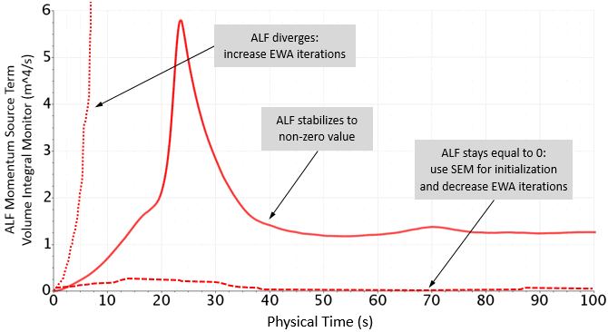
- If ALF diverges, increase the value of EWA iterations.
- IF ALF stays equal to zero, decrease the value of EWA iterations. Additionally, initialize the flow field with turbulent perturbations using the Synthetic Eddy Method. See Setting Up Synthetic Eddy Method.
Typically, 500 to 1000 iterations are enough to get reasonable results.