Operators and Functions
Expressions can use a variety of operations and functions.
Arithmetic Operators
| Operator | Function |
|---|---|
| + | plus |
| - | minus |
| * | multiply |
| / | divide |
Logical Operators
Logical operators allow you to write conditional expressions. See Conditional Expressions.
| Operator | Function |
|---|---|
| == | equal to |
| != | not equal to |
| > | greater than |
| < | less than |
| >= | greater than or equal to |
| <= | less than or equal to |
| && | and |
| || | or |
Trigonometric Functions
Trigonometric functions accept a scalar expression (that is, an expression that evaluates to a scalar) as input, returning a scalar. The input scalar expression can be space or time dependent. If the input depends on space, or time, the returned quantity also depends on space, or time.
In the following table, x and y indicate input scalar expressions. The input scalar expression could simply be a constant value (for example, cos(3.14), sin(6.28)), or an expression that references other scalar quantities (for example, sin(2*${omega}*${Time}), where omega is a scalar parameter and Time is the Time field function).
| Operator | Returns |
|---|---|
| acos(x) | arccosine of x |
| asin(x) | arcsine of x |
| atan(x) | arctangent of x |
| atan2(y,x) | arctangent of y/x |
| cos(x) | cosine of x |
| cosh(x) | hyperbolic cosine of x |
| sin(x) | sine of x |
| sinh(x) | hyperbolic sine of x |
| tan(x) | tangent of x |
| tanh(x) | hyperbolic tangent of x |
Vector Functions
Vector functions accept a vector expression (that is, an expression that evaluates to a vector) as input, returning either a scalar or vector quantity. The input vector expression can be space or time dependent. If the input depends on space, or time, the returned quantity also depends on space, or time.
In the following table, u and v indicate input vector expressions. The input scalar expression could be a constant vector (for example, u = [0.5, 1, 2], or an expression that references other vector quantities (for example, u = ${coefficient}*$${Velocity}, where coefficient is a scalar parameter and Velocity is a vector field function).
When applying the dot or cross vector functions, supply both vectors with reference to the same Cartesian coordinate system.
When plotting vector fields within a vector displayer, the vector is always considered defined in the laboratory Cartesian coordinate system.
| Operator | Returns |
|---|---|
| mag(u) | magnitude of vector u, returned as a scalar |
| mag2(u) | magnitude of vector u squared, returned as a scalar |
| unit(u, x) | unit vector, where x is a scalar that defines the magnitude tolerance.
When the magnitude of a vector is smaller than the specified tolerance, the vector is omitted from the display. |
| dot(u,v) | scalar product of vectors u and v (see Eqn. (5192)), returned as a scalar |
| cross(u,v) | cross product of u and v (see Eqn. (5194)) returned as a vector |
| curl(u) | curl of vector u (see Eqn. (5200)) returned as a vector |
| div(u) | divergence of vector u (see Eqn. (5199)) returned as a scalar |
Symmetric Tensor Functions
Tensor functions accept tensor quantities as inputs, returning either a scalar or vector quantity. In the following table, the field function A represents a 3x3 symmetric tensor :
| Operator | Returns |
|---|---|
|
$$$A.eigValue(<i>),
eigValue($$$A, <i>) |
eigenvalue of , with i=0, 1, 2 (see Eqn. (5209)). Returned as a scalar. |
|
$$$A.eigVector(<i>),
eigVector($$$A, <i>) |
eigenvector of , with i=0, 1, 2 (see Eqn. (5209)). Returned as a vector. |
|
$$$A.trace(),
trace($$$A) |
trace of (see Eqn. (5215)). Returned as a scalar. |
|
$$$A.norm(“infinity”),
norm($$$A, “infinity”) |
infinity norm of (see Eqn. (5218)). Returned as a scalar. |
|
$$$A.norm(1),
norm($$$A, 1) |
1-norm of (see Eqn. (5219)). Returned as a scalar. |
|
$$$A.norm(2),
norm($$$A, 2) |
2-norm of (see Eqn. (5220)). Returned as a scalar. |
|
$$$A.norm(“frobenius”),
norm($$$A, “frobenius”) |
Frobenius norm of (see Eqn. (5221)). Returned as a scalar. |
|
$$$A.mag(),
mag($$$A) |
magnitude of , which is equal to the Frobenius norm (see Eqn. (5221)). Returned as a scalar. |
|
$$$A.mag2(),
mag2($$$A) |
squared magnitude of
:
(see Eqn. (5221)). Returned as a scalar. |
|
Double-dot (double-inner) product of tensors and (see Eqn. (5207)). Returned as a scalar. |
|
Matrix product of tensor and vector (see Eqn. (5204)). Returned as a vector. |
Miscellaneous Functions
In the following table, x and y indicate input scalar expressions.
| Operator | Function |
|---|---|
| ceil(x) | smallest integer not less than x, as a real |
| exp(x) | exponential function, e to the power x |
| abs(x) | absolute value of x |
| floor(x) | largest integer not greater than x, as a real |
| log(x) | base e logarithm of x, natural log |
| log10(x) | base 10 logarithm of x |
| sqrt(x) | square root of x |
| pow(x,y) | x raised to the power of y |
| fmod(x,y) | x modulus y; the floating point remainder of x/y |
| mod(x,y) | equivalent to fmod($x,$y) |
| min(x,y) | the minimum of x and y |
| max(x,y) | the maximum of x and y |
| clamp(x, xMin, xMax) | equivalent to min($xMax, max($x, $xMin)) |
| grad(phi) | gradient of scalar phi returned as a vector (see
Eqn. (5197))
Values calculated using this approach are not necessarily the same as gradients returned from the solvers. This is due to different approaches used in calculating the gradients. In the solvers, a two-pass Gauss algorithm is used, whereas the function provided here uses a least squares approach. Solvers also have more information on boundary values than is available to this function. |
Conditional Expressions
The ternary “?:” operator defines a condition operation if-then-else similar to the C language. For example:
(a > b) ? a : bis equivalent to
z = max(a, b)You can also use parentheses to nest conditional expressions.
Nested conditional expressions allow you to specify different values for a user field function over different time intervals:
($Time <= t_1) ? Value 1 :
(
($Time > t_1 && $Time <= t_2) ? Value 2 : Value 3
)
)
For example, consider a case where the value alternates between 125 and 0 in five-second intervals, and remains at 0 after 15 seconds:
($Time <= 5) ? 125 :
(
($Time > 5 && $Time <= 10) ? 0 :
(
($Time > 10 && $Time <= 15) ? 125 : 0
)
)
The ternary “?:” operator requires all fields to be available on the part (such as the boundary or volume). If one of the fields is not available on the part, then the entire user-defined expression involving the “?:” operator is judged to be invalid and Simcenter STAR-CCM+ fails to fill the field function. In this case, you would see gray in a scene instead of the expected results.
Alternate Value Function
If the value for a scalar or vector expression on a part is not available or computable, you can provide an alternate value for that expression.
Normally Simcenter STAR-CCM+ requires all terms in an expression to exist for the expression to be computable. For example, in the following expression:
$Pressure * $Volumeif Pressure, Volume, or both do not exist for a part, this expression is not computable on that part.
To provide an alternate value, use the alternateValue() operator:
alternateValue($Pressure, 0) * $VolumeIn this example, Simcenter STAR-CCM+ substitutes zero for Pressure if Pressure is not available.
The alternate value operator is not restricted to constants; it can also work with another expression. The syntax for this use of the operator is alternateValue(<scalar/vector expression 1>, <scalar/vector expression 2>), for example:
alternateValue($Pressure1, $Pressure2) * $VolumeIn this example, if both Pressure1 and Pressure2 are not computable, then the alternateValue expression is not computable.
Interpolation of Direction from Parts
The interpolateDirection function generates a field of direction vectors based on the part curves, surfaces, or a filter that you specify. Having a field of direction vectors can be useful when you model anisotropic behavior in materials.
interpolateDirection(@Part("<partname>"), @Representation("<representation>"), @CoordinateSystem("<coordinatesystem>"), <direction>) interpolateDirection(@Filter("<filter>"), @Representation("<representation>"), @CoordinateSystem("<coordinatesystem>"), <direction>)where:
- <coordinatesystem> is the name of a coordinate system in the node in the object tree. The direction vectors are returned based on this coordinate system. If you do not specify a coordinate system, the function uses the default Laboratory coordinate system.
- <partname> is a surface or a curve. For a surface, the direction field is given using the normals of that part. For a part curve, the direction field is given using the line segment directions. If using a surface or a part curve name of a part, the syntax is <partname.surface/curve name>.
- <representation> is the representation that is used to extract the part. It is set in the node in the object tree.
- <direction> defines the orientation of the vectors based on the direction of the normals of the input surface or the direction of the line segment of the input line. Use FORWARD to follow the direction vectors or BACKWARD to reverse the direction vectors.
- <filter> is a filter defined under the node in the simulation tree. The filter can be used to define any compatible objects including multiple part curves or surfaces.
interpolateDirection(@Part("<partname1>::<partname2>::<partname3>"), @Representation("<representation>"), @CoordinateSystem("<coordinatesystem>"),FORWARD) 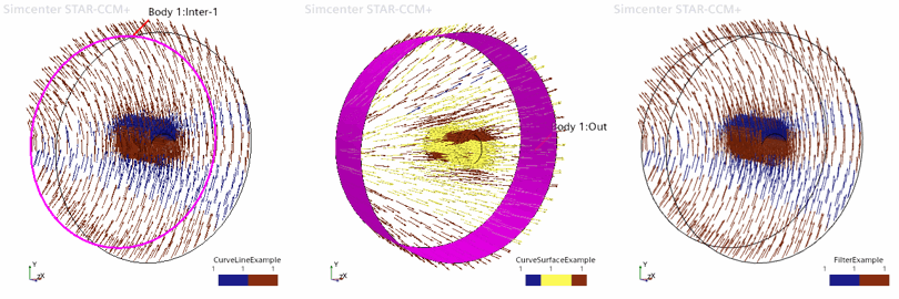
InsidePart Field Function
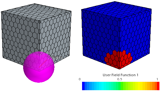
The insidePart function
provides a 0-1 field of values that indicate whether points lie outside (0) or
inside (1) a spatial location described by geometry parts. This function is useful
in defining initial conditions on part of a mesh, for example.
The insidePart function always
returns a value of 0 or 1; 0 indicates points are outside the specified part whereas
1 indicates points are within the specified part. The insidePart
function accepts two types of argument: @GeometryPart and
@Filter.
insidePart
function
is:insidePart(selectorParam, tolerance)insidePart(@GeometryPart("<geometrypart>"))where:
- <geometrypart> is the name of a part within the node in the simulation tree.
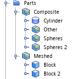
The syntax to identify the cylinder part by name is:
insidePart(@GeometryPart("Composite|Cylinder"))insidePart(@Filter("<filter>"))where:
- <filter> is the name of the filter in the node in the simulation tree. You can create a filter with a
set of conditions and then use the
insidePartfunction with the @Filter argument to find the relevant parts.
| 注 |
|
DistanceToPart and DistanceToSurface Field Function
The distanceToPart and
distanceToSurface functions provide a field of values that
indicate the distance to a given part or part surface.
The distanceToPart
function returns the distance to a part or set of parts. The parts provided to the
function must be closed and manifold.
distanceToPart function is:
distanceToPart(selectorParam, maxSearchDistance)- selectorParam can be either @GeometryPart("<partname>") where partname is the name of the part in the geometry or @Filter("<filtername>") where filtername is the name of a filter within the node.
- maxSearchDistance(optional) imposes a cap on the maximum distance to measure from the target surfaces. Using this parameter provides a performance gain for cases where you are not interested in distances far from the target surfaces.
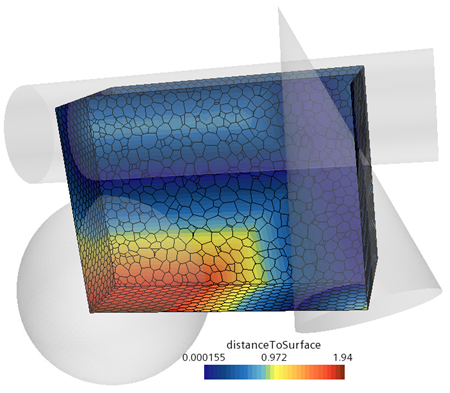
distanceToPart expression is used with a
@Filter argument where the filter returns three parts
(cylinder, cone, and a sphere). The syntax to identify the distance to the parts
is:distanceToPart(@Filter("Parts"))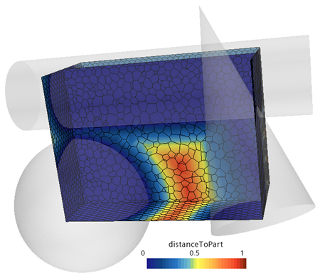
The distanceToSurface
function returns the distance to a part surface. This function allows you to include
parts that are not closed or manifold.
distanceToSurface is:
distanceToSurface(selectorParam, maxSearchDistance)- selectorParam can be one of the following:
- @PartSurface("<partsurfacename>") where partsurfacename is the full path to part surface including any composite parts
- @GeometryPart("<partname>") where partname
is the name of the part in the geometry tree.
distanceToSurfaceautomatically decomposes the part into its constituent part surfaces. - @Filter("<filtername>") where the distance expression is evaluated as the minimum distance to any of the surfaces returned by the filter.
- maxSearchDistance(optional) imposes a cap on the maximum distance to measure from the target surfaces. Using this parameter provides a performance gain for cases where you are not interested in distances far from the target surfaces.
distanceToSurface
expression is different from the distanceToPart expression in two
ways: - It acts on part surfaces and not parts.
- It computes both inside and outside the part
The distanceToSurface field function always uses the root
description of the geometry so it is unaware of any imprint surfaces (which only
impact a later description).
distanceToPart
expression is used with a @Filter argument named
Surfaces which returns the side surfaces of the cylinder and
cone. The syntax to identify the distance to the surfaces is:distanceToSurface(@Filter("Surfaces"))