本案例演示如何使用Fluent材料加工工作区模拟3D注塑吹塑成型（ISBM）过程。该工作区允许设置并求解聚合物ISBM问题，以便可以在给定模具几何形状和规定的操作条件下对物体形状的准确预测。

在本案例中，将学习如何使用Fluent材料加工工作区：

• 设置注塑吹塑成型（ISBM）模拟。
• 计算求解。
• 分析结果，例如生成基于厚度的云图和运行瞬态动画。

1 问题描述

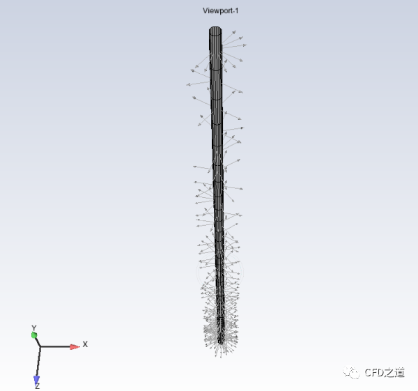
本教程涵盖了3D瓶子的注塑吹塑成型（ISBM）过程。首先将预成型件放入模具中，并通过移动杆进行拉伸。一旦杆到达所需位置（靠近模具底部），则对预成型件施加内压以获得所需的瓶子形状。模型的初始配置如图所示，包括以下三个域：

• 预成型件（以橙色显示）
• 模具（以浅蓝色显示）
• 杆（以浅蓝色显示）

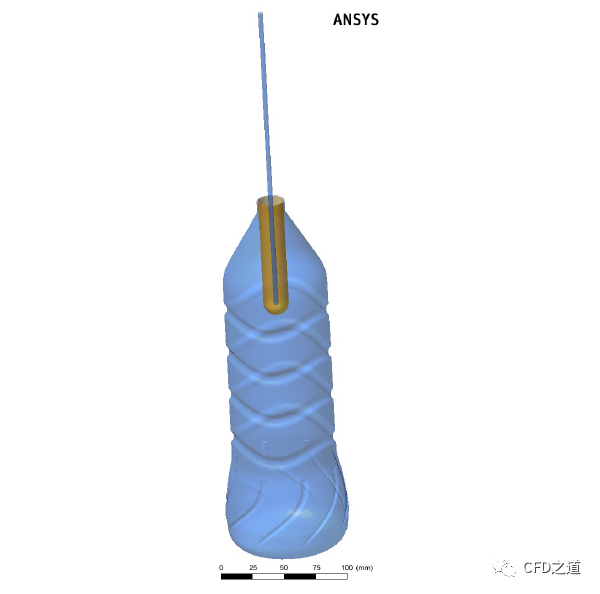
上述区域的尺寸为：

• 杆直径 = 0.02 m
• 杆高度 = 0.1 m
• 模具直径 = 0.097 m
• 模具高度 = 0.3 m
• 预成型件初始厚度 = 0.005 m

模具上可见的凹槽表明该模型不涉及任何几何对称性。

对于这个问题，在施加成型压力时假定预成型件与杆之间的接触释放。在教程设置期间，将使用接触边界条件定义接触释放，并指定单元区域和流体边界条件以考虑以下内容：

1. 在指定时间间隔内杆的速度驱动运动（直到杆达到指定位移）。
2. 施加的成型压力。

此外，在设置期间将指定以下属性：

• 杆向下运动速度 = 0.246 m/s。这种速度确保杆在0.8秒内到达模具内0.2米处。
• 预成型件材料密度 = 1000 kg/m3
• 施加的成型压力 = 1e6 Pa。将定义在0.86秒后施加成型压力。
• 粘附力 = 10 Pa。此值将用于表示预成型件从杆上释放接触。
• 粘度 = 1e5 Pa s

2 设置和求解

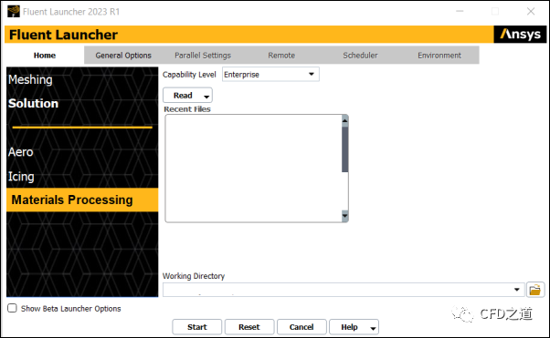
2.1 启动Ansys Fluent

1. 使用Fluent启动器启动Fluent。
2. 在Fluent工作区列表中选择Materials Processing。
3. 点击Start。

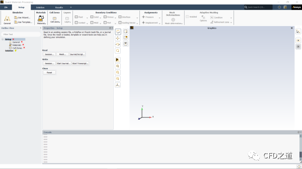
2.2 设置模拟

点击Fluent启动器中的Start将打开Fluent材料加工工作区。

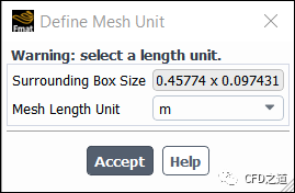
1. 加载提供的网格文件。
1. 在Setup属性下，点击Read下的Mesh… 按钮。
2. 定位并从工作文件夹中选择网格文件（ISBM.msh）。
3. 将Mesh Length Unit设置为m，然后点击Accept关闭对话框。

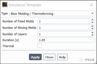
2. 点击按钮Setup → Simulation → Use Template… 打开Simulation Template 对话框设置吹塑模拟
1. 将Type设置为Blow Molding/Thermoforming。
2. 将Number of Fixed Molds设置为1。
3. 将Number of Moving Molds设置为1。
4. 将Number of Layers保持为1。
5. 将Duration设置为1.05秒。
6. 点击 Apply

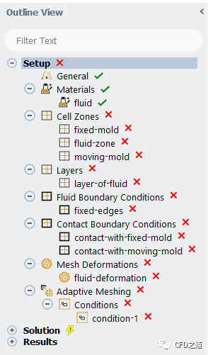
注意大纲视图中状态图标的使用。绿色复选标记表示该对象的属性是满意的。红色’x’表示该对象需要注意。

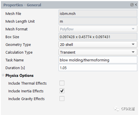
2.3 General属性

点击大纲视图中的 General 节点以显示问题设置的常规设置。对于本教程，保留默认设置。

2.4 材料属性

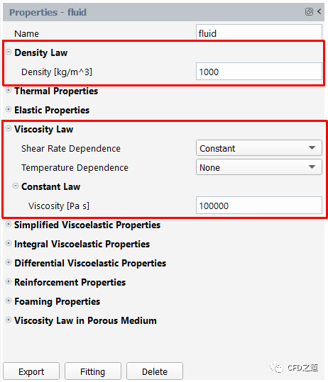
1. 点击模型树节点Setup → Materials → fluid编辑fluid材料的密度和粘度设置
1. 展开 **Density Law **和 Viscosity Law 。
2. 在 Density Law类别中，指定Density为1000 kg/m3。
3. 在 Viscosity Law 类别中，指定Viscosity为1e5 Pa s 。

2.5 单元区域属性

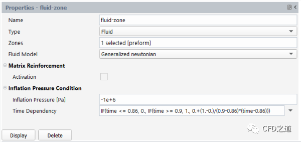
1. 点击模型树节点Setup → Cell Zones → fluid-zone 打开区域设置对话框。

• 对于Zones，选择文本框以打开选择对话框。
• 在选择对话框中，选择preform，然后点击OK以保留选择并关闭对话框。
• 保留对Fluid Model的默认选择Generalized newtonian。
• 输入-1e6 Pa作为Inflation Pressure。
• 点击 Time Dependency条目旁边的箭头，从下拉列表中选择 Expression，然后输入以下表达式作为时间依赖性：IF(time <= 0.86，0.，IF(time >= 0.9，1.，0.+(1.-0.)/(0.9-0.86)*(time-0.86)))。这个表达式对应于一个斜坡函数，在0.86到0.9的时间间隔内从0增加到1。
• 点击 Display 在流体区域上可视化箭头。

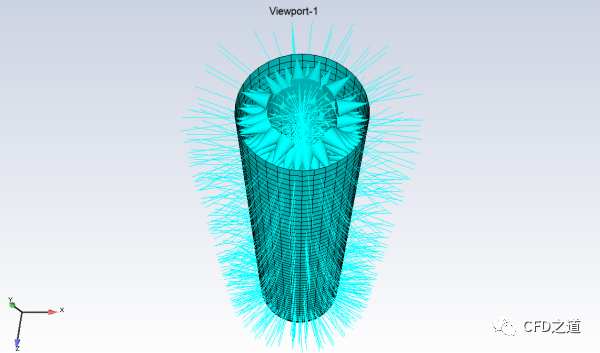
在 fluid-zone 上显示的箭头显示了压力的方向。

2. 定义 fixed-mold 的单元区域属性。

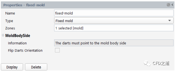
• 鼠标双击模型树节点Setup → Cell Zones → fixed-mold 打开下图所示对话框

• 对于 Zones，选择 mold。
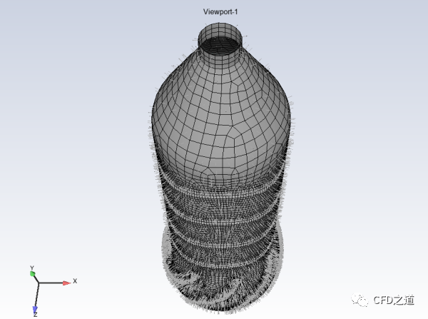
• 点击 Display 在固定模具上可视化箭头。在 fixed-mold上显示的箭头显示方向指向模具本体侧。

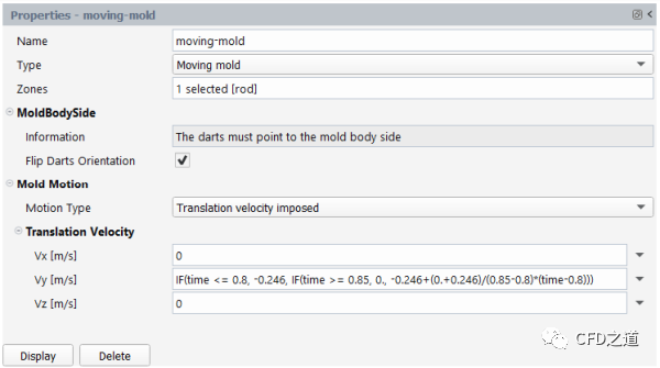
3. 双击模型树节点Setup → Cell Zones → moving-mold 定义 moving-mold的单元区域属性。

• 对于 Zones，选择 rod。
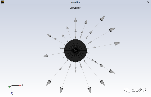
• 点击 Display 在杆（moving-mold)上可视化箭头。

• 在图形窗口中旋转杆以从+Y方向查看箭头。在 moving-mold上显示的箭头指向杆外，它们应该指向杆轴。

• 启用 Flip Darts Orientation选项使箭头指向杆。

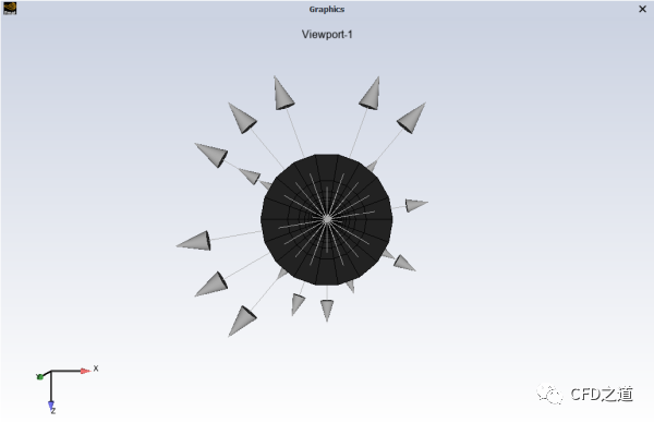
在上图中，飞镖可能仍然看起来朝着杆外。然而，飞镖指向杆轴，但由于缩放与杆几何重叠。

• 点击 Vy 条目旁边的箭头并从下拉列表中选择 Expression，然后输入以下表达式作为Vy:IF(time <= 0.8，-0.246，IF(time >= 0.85，0.，-0.246+(0.+0.246)/(0.85-0.8)*(time-0.8)))。这个表达式对应于一个斜坡函数，在0.8到0.85的时间间隔内从-0.246增加到0。

2.6 层属性

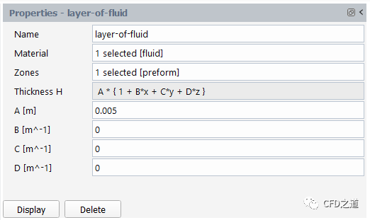
1. 双击模型树节点Setup → Layers → layer-of-fluid 定义layer-of-fluid的属性。
1. 对于Zones，选择右侧的文本框以打开选择对话框。
2. 在选择对话框中，选择preform，然后点击OK以保留选择并关闭对话框。
3. 输入A的厚度0.005 m。

2.7 边界条件属性

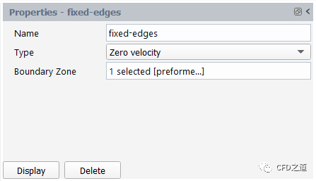
1. 设置fixed-edges边界的条件。
1. 在大纲视图中选择 Fluid Boundary Conditions 下的 fixed-edges以查看此边界条件的模拟。选
2. 选择 Boundary Zone 为 preformedge 。

2.8 接触边界条件

可以使用接触条件来考虑预成型件与固体和移动模具之间的接触。

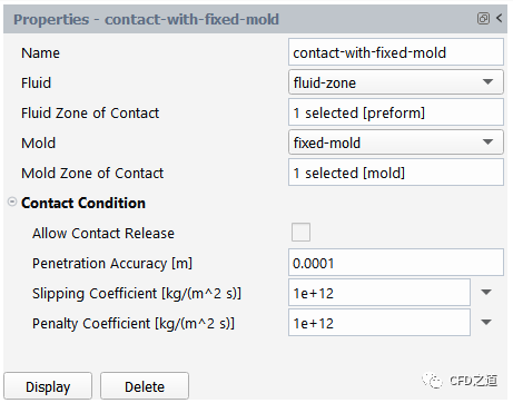
1. 定义预成型件与固定模具之间的接触。
1. 在 **Contact Boundary Conditions **下，选择 contact-with-fixed-mold以编辑此接触条件的默认属性。
2. 选择Fluid Zone of Contact 为 preform 。
3. 选择Mold Zone of Contact 为 mold 。
4. 输入Penetration Accuracy 为 1e-4 m。

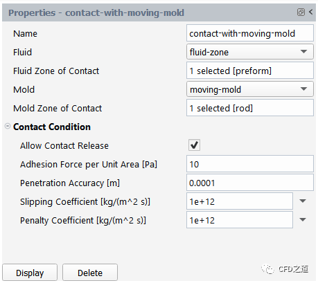
2. 定义预成型件与移动模具之间的接触。
1. 在 Contact Boundary Conditions 下，选择 contact-with-moving-mold以编辑此接触条件的默认属性
2. 选择 Fluid Zone of Contact 为 preform 。
3. 选择Mold Zone of Contact 为 rod 。
4. 输入 Penetration Accuracy为 1e-4 m。
5. 启用 Allow Contact Release选项。
6. 输入 10 Pa作为每单位面积的粘附力。

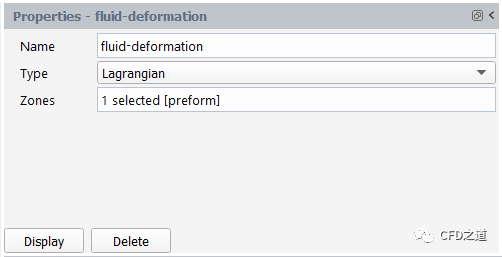
2.10 网格变形属性

这里将预成型件单元区域分配为变形流体。

1. 在 Mesh Deformations 下，选择 fluid-deformation以编辑模拟中流体变形区域的默认属性。
2. 将变形类型保留为Lagrangian。
3. 对于Zones，选择preform。

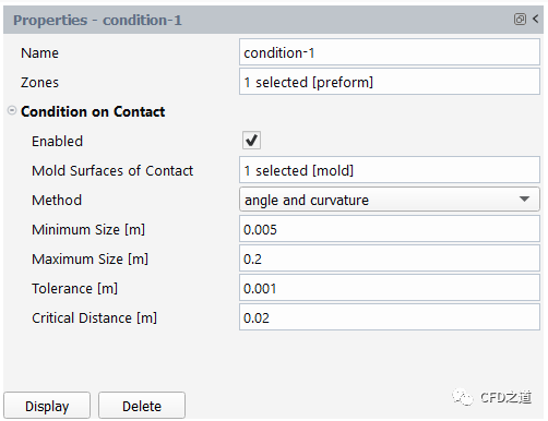
2.11 自适应网格设置

定义自适应网格化的条件和设置，用于在求解过程中细化网格。

1. 选择模型树节点Setup → Adaptive Meshing → Conditions → condition-1定义自适应网格条件（condition-1）。
1. 选择Zones 为preform。
2. 选择Mold Surfaces of Contact 为mold。
3. 保留Method 为angle and curvature。
4. 输入Minimum Size 为0.005m。
5. 输入Maximum Size 为0.2 m。
6. 输入Tolerance 为 0.001m。
7. 输入Critical Distance 为0.02 m。

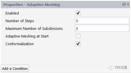
2. 选择Setup → Adaptive Meshing编辑自适应网格化属性。
• 输入Number of Steps 为5。

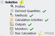
2.12 解决方案

打开大纲视图的 Solution 分支（或使用Ribbon）。在这里可以查看问题设置和其他求解属性。大多数项目表明当前默认值是合适的。

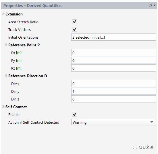
1. 点击节点Solution → Derived Quantities编辑 Derived Quantities。
1. 在 Extension 下，启用 Track Vectors 选项以显示其他选项。
2. 对于 Initial Orientation，选择 initially parallel to D 和 initially perpendicular to D。
3. 对于参考点 Px，Py，和 Pz，保留输入0m。
4. 输入参考方向 Dir-x 为0。
5. 输入参考方向 Dir-y 为1。
6. 输入参考方向 Dir-z 为 0。
7. 启用 Self-Contact，并保留对 Warning 的选择，以便在检测到自接触时执行操作。

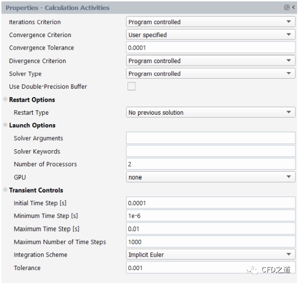
2. 点击节点Solution → Calculation Activities 编辑 Calculation Activities
1. 选择 Calculation Activities，查看可用选项。
2. 在下拉列表中，从 Convergence Criterion，选择 User specified
3. 输入 0.0001作为 Convergence Tolerance
4. 输入 1e-4秒作为 Initial Time Step
5. 输入 1e-6秒作为 Minimum Time Step
6. 输入 1e-2秒作为 Maximum Time Step
7. 输入 0.001作为 Tolerance

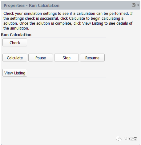
3. 点击节点Solution → Run Calculation检查的问题设置。
1. 点击 Check，查看模拟设置。Fluent将提示设置是否存在任何问题，并提供求解指导。

4. 计算求解
1. 点击 Calculate，开始计算。
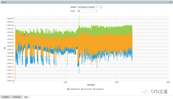
2. 点击 Plots，查看收敛监视器的图表。
3. 计算完成后，在Transcript标签页中检查求解列表，确认其成功。

5.保存工作。

使用菜单File → Write → Session...，输入 ISBM，作为会话名称保存文件。

3 结果

使用大纲视图或Ribbon中的 Results 部分中的各种工具查看结果，可以设置分布、矢量等。

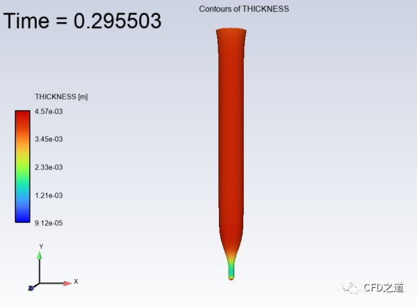
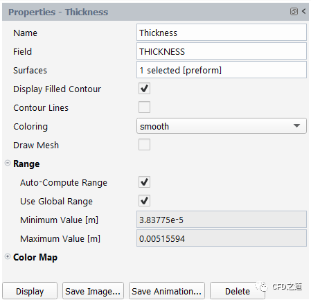
1. 点击Results → Graphics → Contour → New…显示 preform 表面的厚度（THICKNESS）分布。

• 指定一个新的 Name (Thickness)。
• 对于 Field，选择 THICKNESS。
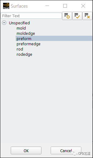
• 对于 Surfaces，选择该字段以打开 Surfaces 对话框，在其中可以选择相关边界。从列表中选择 preform，然后单击 OK 关闭对话框。

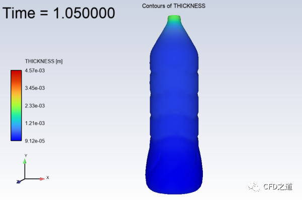
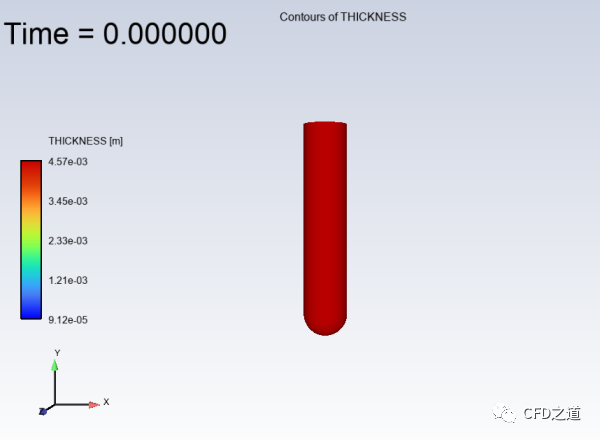
• 保留其余默认值，然后单击 Display 在图形窗口中查看厚度分布图。

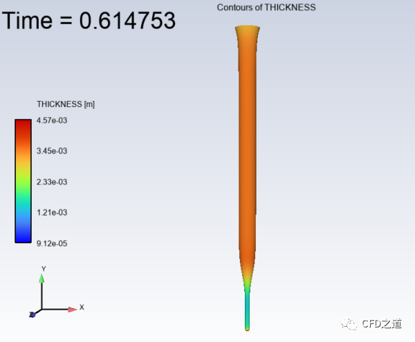
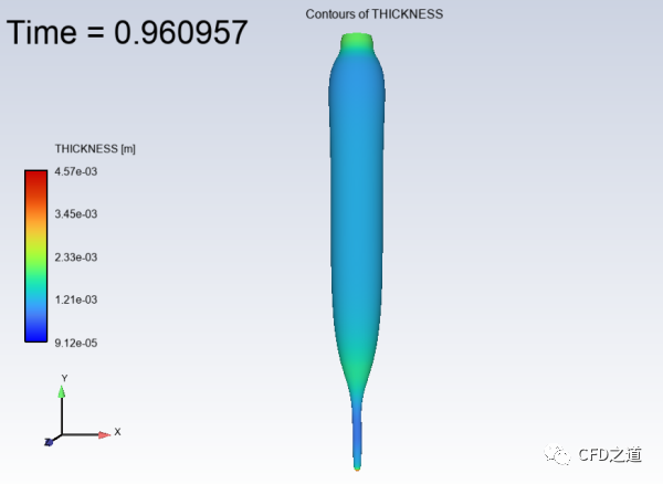
2. 点击按钮Results → Timestep 查看 THICKNESS 分布的动画。

• 要重置时间步长，请将当前动画时间步长值更改为 0。或者也可以将滑块移动到最左端，或单击 Jump to Start 按钮。
• 要开始动画，单击 Play 按钮
• 要停止动画，单击 Stop 按钮

3. 点击Results → Graphics → Contour → New… 显示面积拉伸（AREA_STRETCH）的分布，用于 preform 表面。

重复前面的步骤，在 preform 表面上创建一个新的分布，其名称为 AreaStretch，其物理量设置为 AREA_STRETCH。

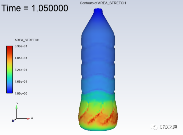
重复前面的步骤查看分布的动画。

4. 点击Results → Graphics → Contour → New…显示自接触（SELF_CONTACT）的分布，用于 preform 表面。

重复前面的步骤，在 preform 表面上创建一个新的分布，其名称为 Self-contact，其物理量设置为 SELF_CONTACT。

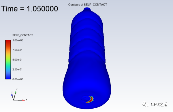
重复前面的步骤可以查看动画。

注：本案例为Fluent Workspace Tutorials，案例输入文件可从官网下载。

（完）

​